Vortex Panel Method Solver for Airfoil Aerodynamics
Boundary-integral potential flow from raw airfoil coordinates, solved by Gauss elimination
- Role
- Sole author
- Status
- Completed
Headline results
Why potential flow still earns its place
Under the assumptions of inviscid, incompressible, steady, irrotational flow, the governing equations collapse to Laplace's equation for a velocity potential. Solutions are then dictated entirely by boundary conditions, which makes airfoil aerodynamics a classic boundary value problem.
The appeal is computational: because the flow satisfies Laplace's equation everywhere except on the body surface, the problem reduces from a two-dimensional field solve to a one-dimensional boundary discretization. Panel methods resolve surface pressure and lift with orders of magnitude fewer degrees of freedom than a grid-based Euler or Navier–Stokes solver, which is why they still sit inside modern industrial design loops as fast aerodynamic predictors.
Setting up the solve
The airfoil surface is discretized into N straight panels, each carrying an unknown constant vortex strength. Enforcing no-penetration at each panel control point requires computing the velocity every panel induces at every other control point, which assembles into a dense influence matrix. Because the induced velocity from each vortex element is analytic via Biot–Savart, the whole problem reduces to a finite linear system.
I solved it with Gauss elimination — normalize each diagonal, eliminate the rest of the column, continue to the identity — following the algorithm from Numerical Recipes and course lecture notes. It is robust and well suited to the relatively small dense systems a panel discretization produces.
One correction along the way is worth recording. My initial project outline called for Gauss–Seidel relaxation, on the assumption that the vortex strengths acted as boundary conditions for a field-based potential solve. That interpretation was wrong. In the classical vortex panel method the flow is represented entirely by discrete vortex elements on the surface, and the strengths are coefficients in a linear superposition of analytically known velocity fields — not boundary data for an elliptic solver. Iterative relaxation is not required at all. Gauss–Seidel stays relevant for potential flow problems solved on a spatial grid; the panel method bypasses the grid entirely.
Results and what went wrong
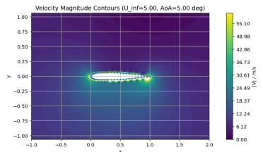
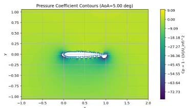
Velocity magnitude and pressure contours for a NACA 0012 at positive angle of attack came out qualitatively correct — the acceleration over the upper surface and the pressure signature of a lifting airfoil are both clearly present. The lift magnitudes were not.
| Angle of attack | Circulation Γ | C_L (computed) |
|---|---|---|
| −5.00° | −86.93 | −34.77 |
| −2.00° | −34.81 | −13.92 |
| 0.00° | 0.00 | 0.00 |
| 2.00° | 34.81 | 13.92 |
| 5.00° | 86.93 | 34.77 |
| 8.00° | 138.82 | 55.53 |
| 10.00° | 173.20 | 69.28 |
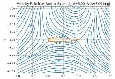
Those C_L values are unphysically large, and the flow field showed non-physical recirculation downstream of the airfoil. Both point to the same cause: the circulation being solved for is not consistent with a clean Kutta-enforced trailing-edge flow.
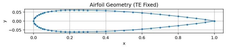
The primary limitation is the trailing-edge formulation in the coordinate files themselves. Many public airfoil coordinate sets do not provide a single, perfectly shared trailing-edge point — the final upper-surface and lower-surface points may not coincide. Panel methods are acutely sensitive to this, because the Kutta condition is fundamentally a constraint at the trailing edge. Even with a preprocessing step that averages the endpoints into a shared point, the resulting last panels can become nearly collinear, extremely short, or poorly oriented, degrading the conditioning of the influence matrix and distorting tangential velocity near the trailing edge.
Four fixes, in order
- 01Use a tangential-velocity Kutta condition rather than a simple trailing-edge strength sum — enforce equal tangential velocity on upper and lower surfaces, or continuous pressure. This is physically aligned with finite velocity at a sharp trailing edge and behaves better than a relation between two panel strengths.
- 02Introduce a wake panel as an additional unknown, so the wake carries net circulation downstream in a controlled, physically interpretable way. This typically improves both conditioning and streamline realism.
- 03Switch to a linear-strength vortex sheet near the trailing edge, letting sheet strength vary along each panel and making the Kutta constraint cleaner to express.
- 04Improve the trailing-edge geometry before solving — enforce a true single node, re-sample with a controlled point distribution near the trailing edge, and remove near-duplicate points so the last panels are not degenerate.
The implementation demonstrates the full pipeline — panel setup, influence matrix, direct solve, post-processing, visualization. What the non-ideal results establish is that trailing-edge discretization and the specific Kutta implementation dominate the accuracy of a panel method, which is a more useful finding than a clean answer from a curated geometry would have been.