Wind-Turbine Blade Aerodynamic Load & Flapwise Deflection Model
Blade element momentum theory, Green's-theorem section properties, and a piecewise Euler–Bernoulli solver
- Role
- Sole author — aerodynamic model, section-property routine, and beam solver
- Status
- Completed
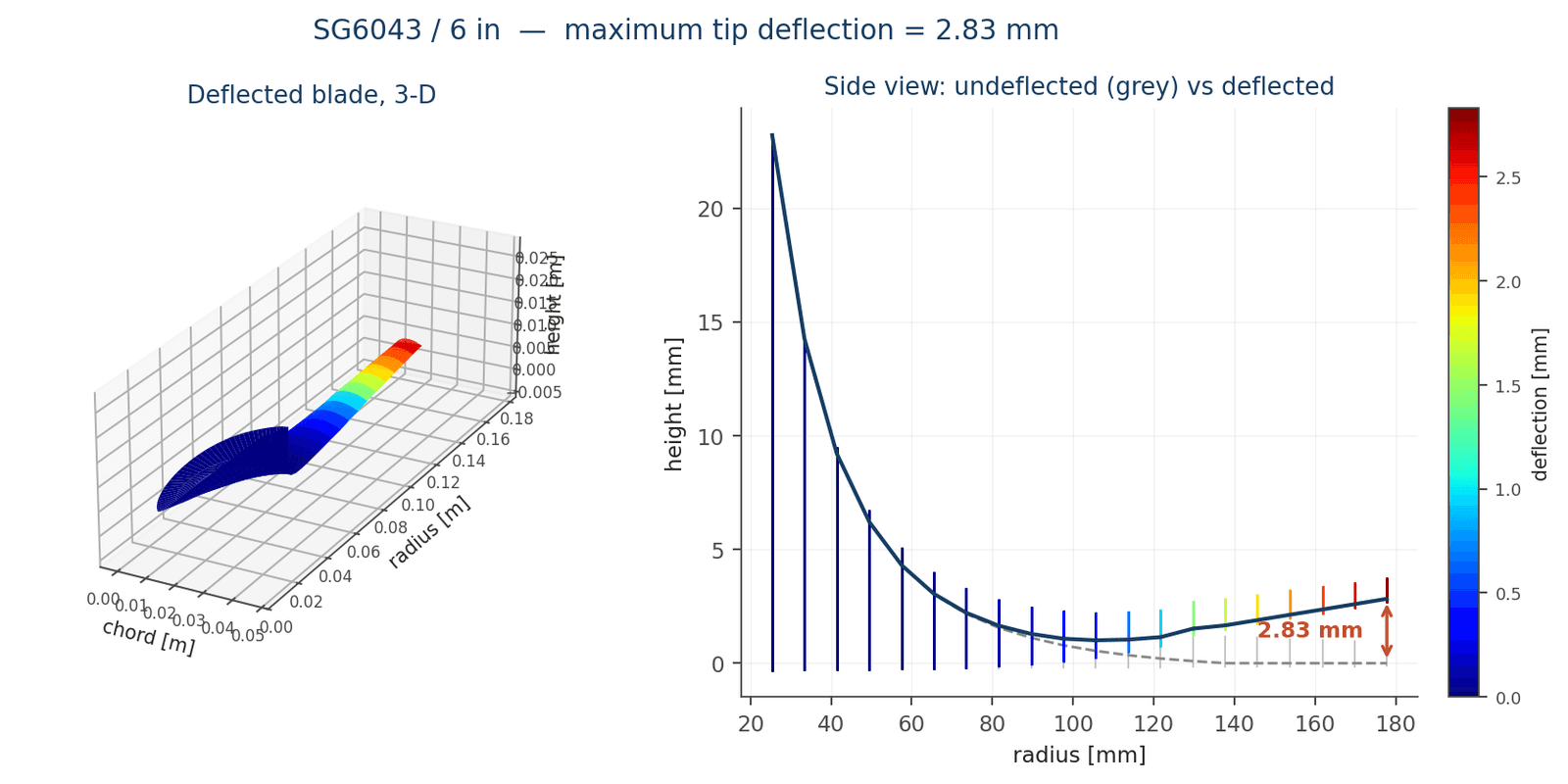
Headline results
Scope and motivation
A three-intern team overhauled Cornell's Wind Tunnel Studio and then exercised the rebuilt “Big Blue” tunnel the way its users would — designing, 3D-printing, and testing small wind-turbine blades. The Betz blade model behind the printed geometry was a team effort; measured peak power came in roughly 22% below prediction.
To test whether blade flex explained that gap, I wrote this load-and-deflection model from scratch on my own — the aerodynamic force model, the section-property routine, and the beam solver. It takes airfoil polars and a blade planform and returns the deflected shape of a single blade under its own aerodynamic load.
Governing equations — aerodynamic load
The blade is cut into 20 annular elements. For each, blade element momentum theory requires that two independent statements of the same element load agree. Momentum theory applies the Rankine–Froude actuator-disk and angular-momentum balances to the annulus; airfoil theory builds the same load from tabulated lift and drag on the local section.
Here u = U₁(1−a) is the axial velocity at the disk and w = Ωr(1+a′) the tangential, with B = 3 blades. Both closures are annulus totals across all blades, so a single cantilevered blade carries T/B.
Solved as a constrained minimisation
Rather than the usual fixed-point iteration on the induction factors, I posed the closure as a bounded nonlinear minimisation and handed it to fmincon at each of the 20 stations.
- The R factor on the thrust residual puts both terms in N²·m², so the cost is dimensionally homogeneous and neither residual is implicitly weighted by unit choice.
- A warm start of a₀ = [a_min, 1/3] seeds the tangential factor at the Betz optimum.
- Bounds a ∈ [a_min, 0.5] keep the solver out of the turbulent-wake state where momentum theory is invalid; a_min comes from streamtube continuity against the tunnel wall.
- Optimality and step tolerances at 1×10⁻¹⁰, so residuals converge essentially to zero.
From distributed load to a deflected beam
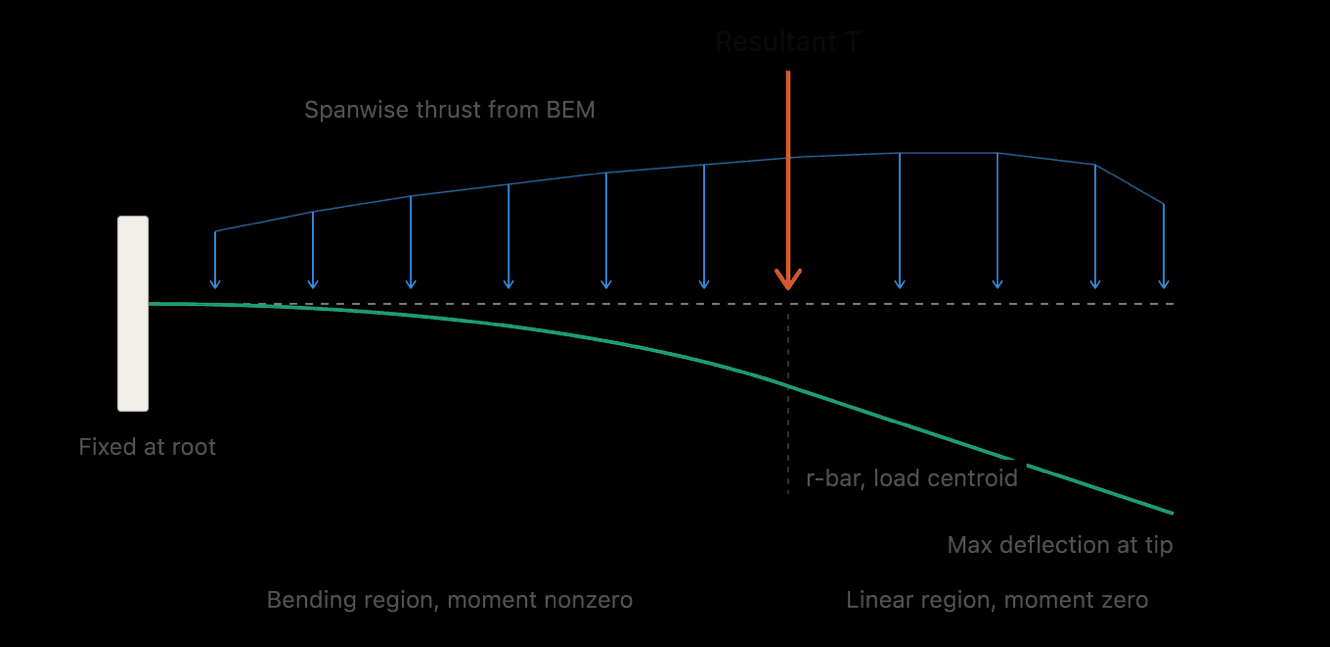
The blade is treated as a cantilever fixed at the root and loaded in the flapwise direction. The spanwise distribution is collapsed to a statically equivalent point force using the standard equivalence — equal resultant and equal first moment about the root. This is exact for the internal moment inboard of the load centroid, and it is what makes the rest of the integration analytic rather than numerical.
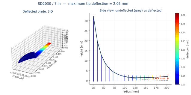
Because I varies along the span, one pair of constants cannot serve the whole blade. The solver walks slice by slice and re-solves C₁ and C₂ at every interface to enforce C⁰ and C¹ continuity — matching both displacement and slope across each boundary. The clamped root supplies v = 0 and v′ = 0 to seed the first slice. Outboard of the load centroid the moment vanishes, v″ = 0, and the shape is exactly straight, so maximum deflection always falls at the tip.
Section stiffness from the true airfoil contour
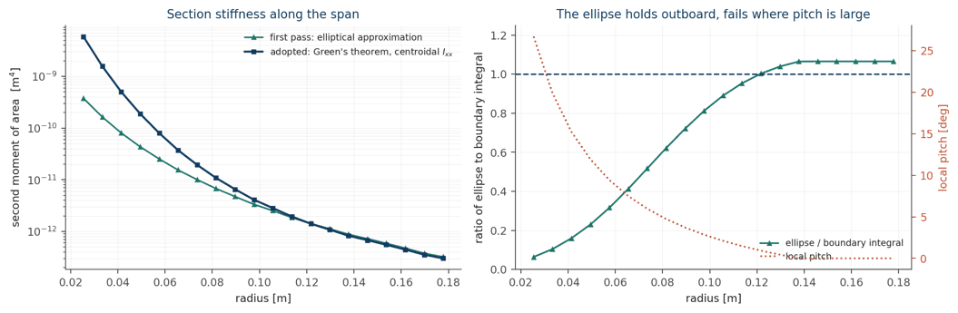
The stiffness EI needs the second moment of area of every airfoil section along the span. My first pass approximated each section as a solid ellipse of semi-axes a = c/2 and b = t/2, giving I = πab³/4. It is cheap, closed-form, and adequate where the section sits close to level.
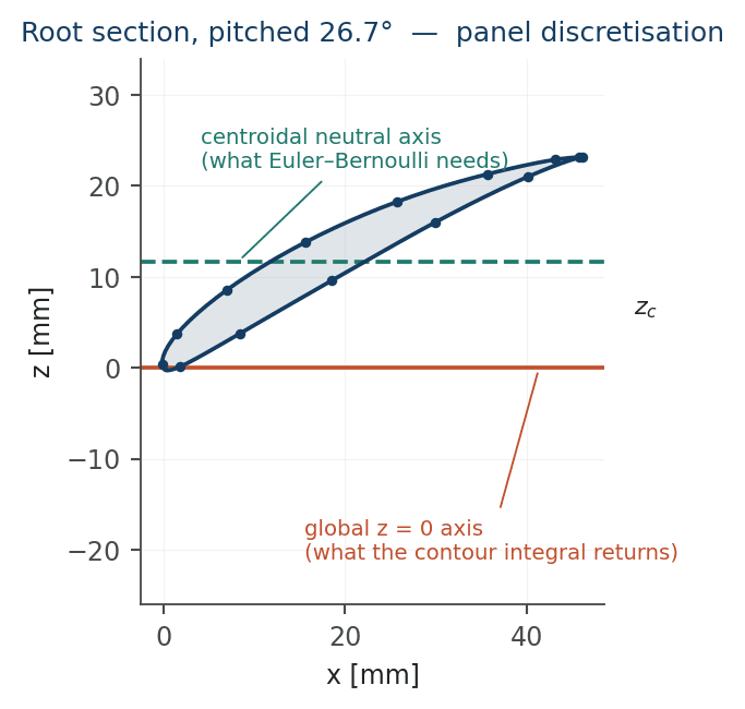
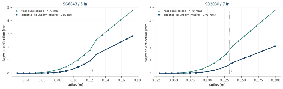
Its weakness is that it takes the section as drawn and ignores the pitch rotation entirely. A section twisted 26.7° at the root presents a far greater depth about the flapwise bending axis than its unrotated thickness suggests, so the ellipse understates stiffness badly exactly where the bending moment is largest. It holds to within 7% outboard where pitch approaches zero, but runs 16× low at the root — and carries a 69% error through to the predicted tip deflection.
I replaced the approximation with a boundary integral over the actual Selig coordinate polygon, taken in its rotated attitude. The area vector field F = (−z/2, x/2) has two-dimensional curl equal to 1, so its contour integral returns the enclosed area. Weighting that same integrand by zⁿ and re-applying Green's theorem yields a family of moments from a single loop.
Each panel is integrated with two-point Gauss–Legendre quadrature. Along a straight panel the n = 2 integrand is cubic in the panel parameter, and two-point Gauss is exact through cubics — so for a polygon the routine is exact rather than merely convergent. Euler–Bernoulli needs the second moment about the section's own neutral axis, not the global reference line, so the centroid comes from the same loop and the parallel-axis term is removed. At the 26.7° root station that parallel-axis term is 81% of the raw value.
Verification
| Check | Method | Result |
|---|---|---|
| Section routine | Green's-theorem result against the closed-form shoelace polygon integral, all 20 stations. | Max relative error 1.0×10⁻¹⁴ (SG6043) and 1.8×10⁻¹⁴ (SD2030) — machine precision. |
| Load magnitude | Rotor thrust against the actuator-disk limit: 1.3700 N over a 0.09931 m² swept area at 5 m/s. | C_T = 0.931, inside the theoretical maximum of 1.0. Confirms the closures return annulus totals. |
| Section model | Elliptical approximation against the boundary integral, station by station, versus local pitch. | Within 7% outboard; 16× low at the 26.7° root. Worth 69% on the final tip deflection. |
The first check matters because the boundary integral is the one place in the chain where a sign or constant slip would be invisible in the output — the deflection would simply come out plausible and wrong. Comparing against an independent closed form on the same polygon removes that risk. The second is a physical bound rather than a numerical one: no actuator disk can exceed C_T = 1, so a rotor coefficient of 0.931 confirms both that the BEM closure returns annulus totals across all three blades and that dividing by B before loading the cantilever is the right move.
Results
| Quantity | SG6043 / 6 in | SD2030 / 7 in |
|---|---|---|
| Operating point | 366.52 rad/s (λ = 13.03) | 172.24 rad/s (λ = 7.00) |
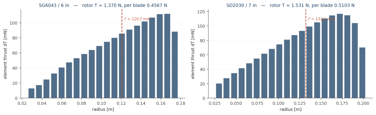
| Rotor thrust, 3 blades | 1.3700 N | 1.5309 N |
| Thrust per blade | 0.4567 N | 0.5103 N |
| Load centroid r̄ | 0.1207 m | 0.1322 m |
| Rotor power | 1.506 W | 1.182 W |
| Max tip deflection, PLA (E = 2.80 GPa) | 2.828 mm | 2.051 mm |
| Max tip deflection, ABS (E = 2.28 GPa) | 3.473 mm | 2.519 mm |
Assumptions and limitations
- Linear elastic, isotropic, homogeneous solid cross-section. An FDM-printed part is infilled and layer-direction anisotropic, so the effective flapwise modulus is lower and orientation-dependent.
- Small deflection: no geometric stiffening, and no follower-force effect as the blade bends out of the wind.
- No centrifugal stiffening. At 3500 rpm this is the dominant missing restoring term, so the prediction is conservative.
- Pure flapwise bending — the product of inertia is discarded, so coupled lead-lag deflection and bend-twist behaviour of the highly pitched inboard sections are not captured.
- Load frozen at the rigid geometry: no aeroelastic feedback from the deflected shape back into the BEM solve.
- Clamped boundary conditions applied at the midpoint of the first element, so the inboard 3.8 mm of blade sits outside the integration.
The two changes that would most improve fidelity, in order: add the centrifugal stiffening term to the moment balance, and iterate the BEM solve on the deflected geometry so load and shape converge together.