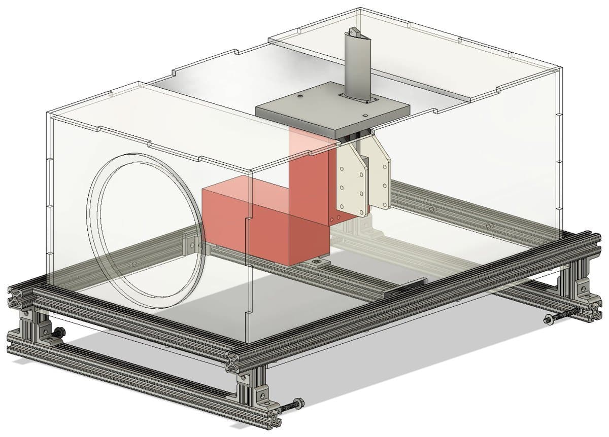
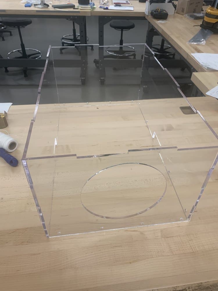
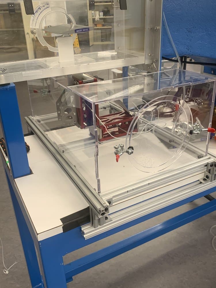
Hot-Wire Anemometry Traverse for the “Big Blue” Wind Tunnel
Design, fabrication, and test-section velocity characterization
- Role
- Individual project within a three-intern studio overhaul
- Status
- Built & Commissioned
Headline results
Context: one part of a studio-wide equipment overhaul
The Wind Tunnel Studio serves faculty, researchers, students, and project teams through four low-speed tunnels — three smaller “Baby Blue” tunnels for airfoil lift and drag, and one larger “Big Blue” tunnel for wind-turbine testing. All four had aged into producing invalid data. Over one summer, a three-intern team overhauled the studio's hardware and curriculum through four parallel efforts.
- 01Load-cell diagnosis — ran airfoil lift/drag campaigns against the tunnels' built-in force sensors and traced the invalid data to faulty load cells.
- 02Load-cell replacement — swapped the cells and designed, machined, and built a new modular mount for them.
- 03Speed-measurement redesign (this project) — I owned the replacement of the tunnel's fixed, immobile pitot-static probe with a hot-wire traverse.
- 04Wind-turbine campaign — exercised the rebuilt tunnel the way its users would, with MATLAB modeling to compare measured against predicted performance.
Design goals
- 01Measure freestream speed far more accurately — and more informatively — than the fixed pitot-static probe it replaced.
- 02Resolve velocity at many points across the tunnel cross-section, not just one location.
- 03Be maneuverable: removable and repositionable to preset cross-section locations, so users can read the flow fore and aft of a turbine during a campaign, and so it lifts out for repair.
- 04Occupy minimal frontal area so it barely disturbs the flow — its wake must fully redevelop before reaching a turbine mounted aft of the probe.
- 05(Self-imposed) minimize cost by using in-house equipment wherever possible.
- 06Be designed and built within a deadline of less than one month.
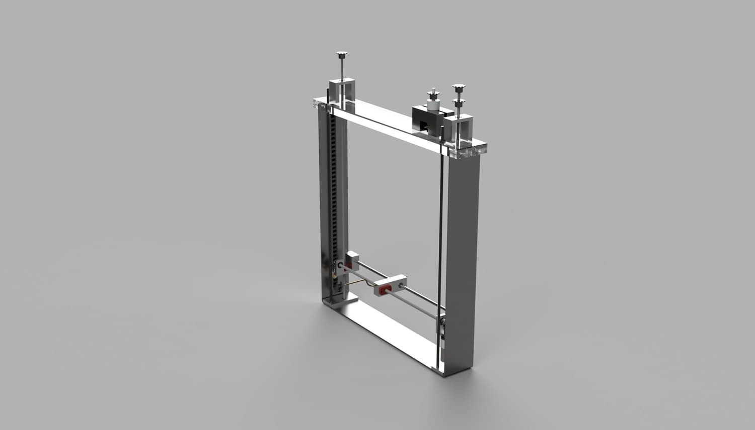
Concept trade study
I sketched four drive concepts and weighed them on cost, goal fit — above all deterministic positioning and low frontal area — build time, and simplicity.
| Drive concept | Pros | Cons |
|---|---|---|
| Cable-and-pulley (prototype) | Cheapest; fewest parts; simplest to build; very low frontal area. | Cable slips on the pulleys — position is neither deterministic nor repeatable; tension and stretch drift. Fails the known-point survey goal. |
| Timing-belt drive | Positive toothed grip (no gross slip); fast; inexpensive; low friction. | Belt stretch and compliance under load degrade repeatability; needs tensioning; pulleys add bulk. |
| Rack-and-pinion | Positive engagement; robust over long travel; moderate cost. | Gear backlash unless preloaded; the rack adds cross-sectional bulk in the flow; more wear and noise. |
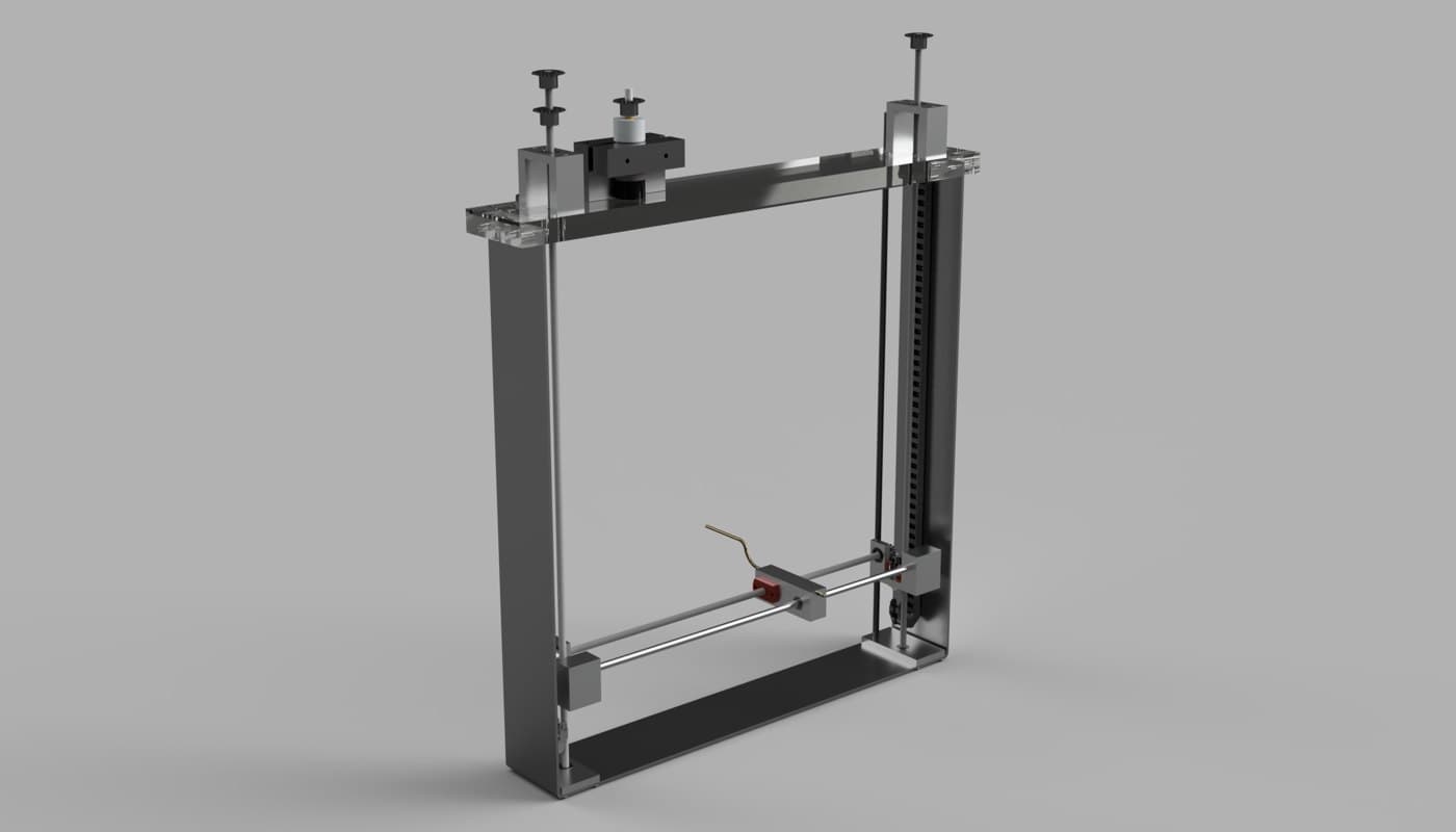
| Lead-screw + rails (chosen) | Rotation maps rigidly to linear travel — no slip; resolution and repeatability together; compact frontal area; small in-house motors suffice; self-locking, holds position. Spare lead screws already in-house. | Needs careful alignment; screw whip at length, handled with support bearings. |
Fabrication & drivetrain
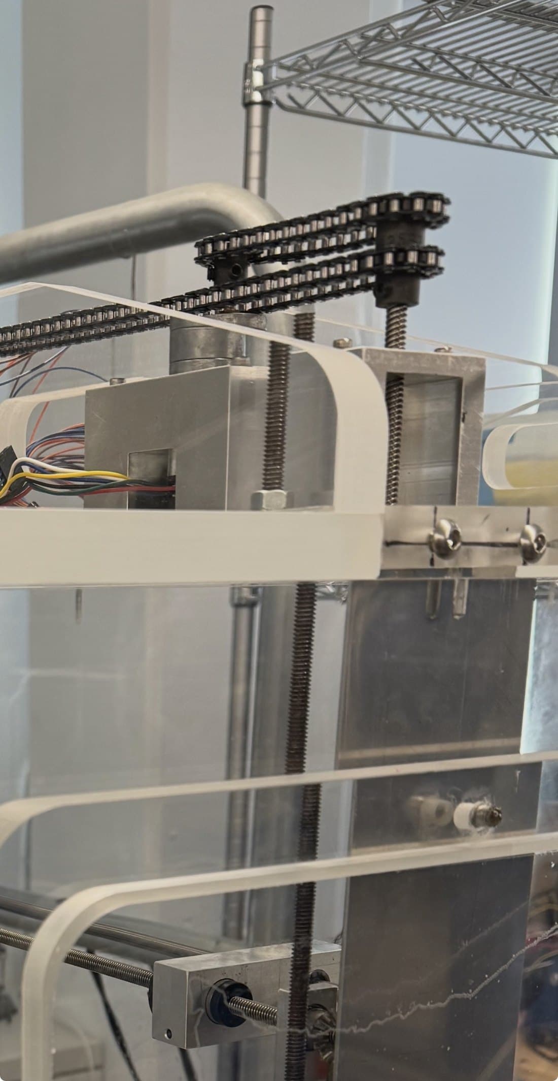
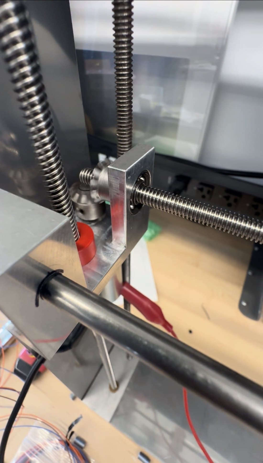
Geared DC motors with built-in positional encoders drive two Thomson precision lead-screw axes through miter gears and an ANSI-25 chain; igus cable chain manages the wiring. I split fabrication by tolerance class rather than by convenience.
| Part / material | Fabrication method |
|---|---|
| Motor and lead-screw mounts | Machined in-house by me on the mill |
| Motor-to-miter-gear adapters | Resin printed |
| Horizontal motor mounts | Routed to a professional machinist |
| 10-gauge stainless steel frame | Welded by a professional machinist |
Instrumentation & integration
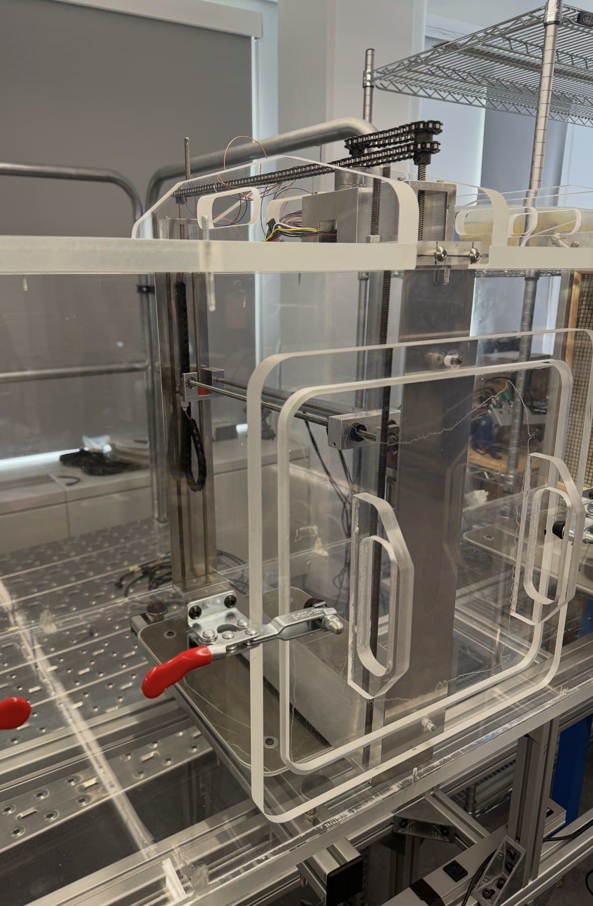
The traverse mounts directly on Big Blue with the probe in the measurement plane. After wiring the data-retrieval circuit to the sensor manufacturer's recommendation, I built a LabVIEW VI as the operator interface and connected it to an Arduino Uno handling hardware I/O — so every surveyed point pairs a commanded (x, y) coordinate with a recorded velocity.
Design validation
I validated the design three ways, each isolating a different failure mode. First, free-body diagrams of the lead screws and mounts sized the motor torque needed to drive each axis against friction and load. Second, an ANSYS CFD simulation of the carriage wake confirmed the flow fully redevelops downstream of the traverse before reaching a turbine mounted aft of it — directly satisfying goal 4. Third, empirically: I mapped the full test-section cross-section and then ran a complete mock wind-turbine campaign as the studio's users would.
Results: test-section velocity survey
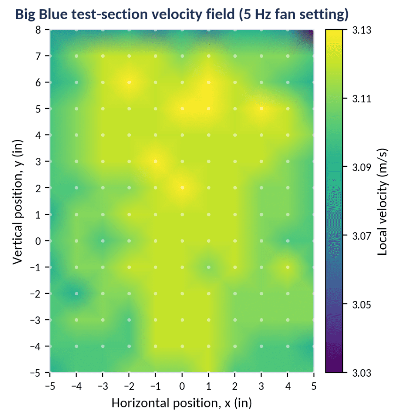
Traversing an 11 × 14 grid — 154 points at 1-inch spacing — at a 5 Hz fan setting, the mapped field is uniform: mean 3.11 m/s, standard deviation 0.44% of mean, peak-to-peak ±1.6%. That variation sits at the level of the hot-wire's own scatter, so there is no resolvable large-scale non-uniformity in the core.
Exercising the tunnel: wind-turbine campaign
With trustworthy speed measurement in place, the team ran Big Blue end to end the way its users would — designing, printing, and testing small wind-turbine blades to expose whatever faults remained. Blade design came from a MATLAB sweep of 24 NACA airfoils against a Weibull wind-speed distribution, converging on a NACA 4415 optimized for 5.5 m/s and 1500 RPM. Power curves were then measured through the team's LabVIEW VI while stepping a torque brake through rotation rates.
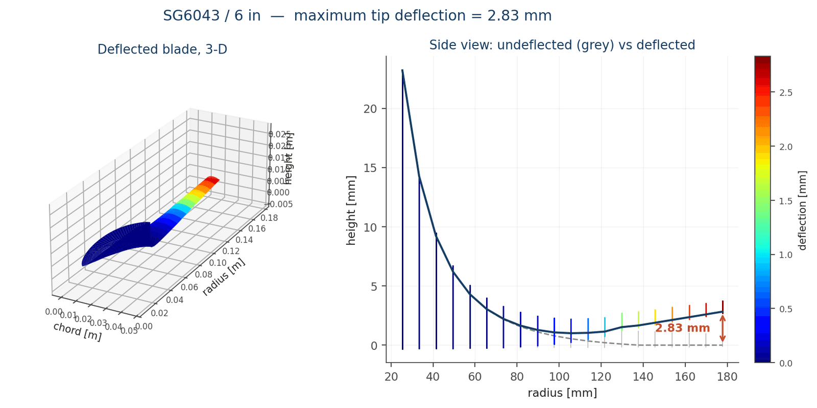
The campaign surfaced concrete limitations: blades ran over 4–7 m/s versus the predicted 3–8 m/s; near the 2,000 RPM structural limit the turbine stalled rapidly; inconsistent brake stepping left unevenly spaced data; and measured peak power came in roughly 22% below prediction. That last gap is what sent me to build a blade load and deflection model from scratch to test whether blade flex could explain it.
Alongside: load-cell diagnosis and modular mount
The same summer, I helped root-cause the invalid lift and drag data in the Baby Blue tunnels: verified airspeed via pitot-static calibration cross-checked against barometric measurement, recalibrated the legacy load sensor, and isolated the fault to the load cell itself, which was unrepairable. I then designed the replacement's modular 80/20 mount with a manufacturer-recommended acrylic shield isolating the sensor from flow disturbance; a stinger carries airfoil loads from the test section down to the shielded cell.