Long-Range Glider Design & Competition
Designing for Earth, scaling for a fictional atmosphere, and flying against thirty other teams
- Role
- Team of three
- Status
- Top 5 Finish
Headline results
The brief
Design a long-range, slow-flight glider for the atmospheric conditions of a fictional planet — thinner air, lower gravity, a lower speed of sound — and then design a companion Earth glider that reproduces the same non-dimensional flow behaviour so the design can actually be tested here. Two aircraft, one set of matched Reynolds and lift coefficients.
Airfoil and wing selection
Rather than picking an airfoil by reputation, we benchmarked full-scale sailplanes on the metrics that actually matter for the mission — aspect ratio, minimum sink rate, maximum lift-to-drag, and best glide ratio — and worked backwards from the best performer. The Alexander Schleicher ASW-22 stood out: aspect ratio 32.47, minimum sink 0.44 m/s, maximum L/D of 62, best glide ratio 54.
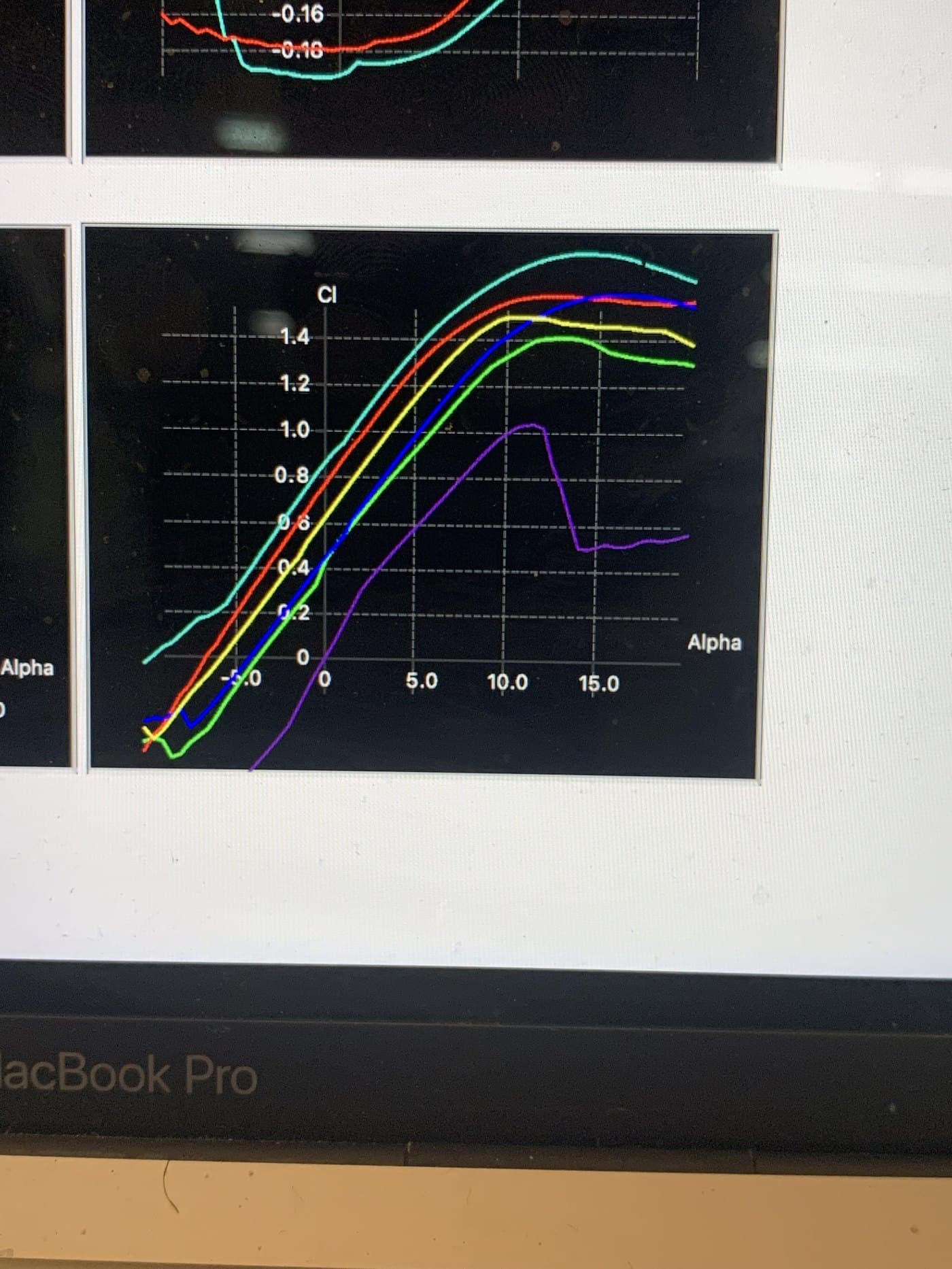
Low sink rate keeps the glider airborne longer; high glide ratio converts that time into distance. Aspect ratio then tells you what it costs structurally to chase that performance. The ASW-22 uses a Horstmann and Quast HQ-17/14.38 section, so that is where we started, reading published polars at the Reynolds number our much smaller aircraft would actually see — around 26,000, two orders of magnitude below the full-scale aircraft.
The low-Reynolds polars are worse than the full-scale ones, but our glider is small and light and does not need to generate as much lift, so a lower lift coefficient is acceptable provided drag falls with it. The HQ-17 keeps a relatively high C_l/C_d for a glider this small, which is why we stayed with it.
Configuration decisions
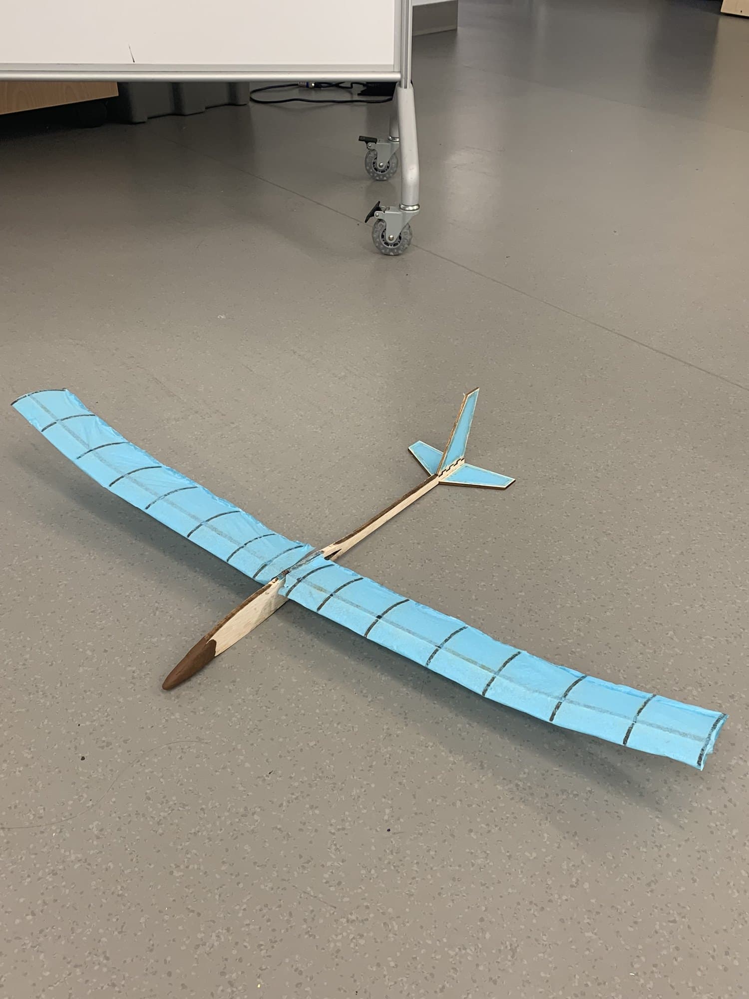
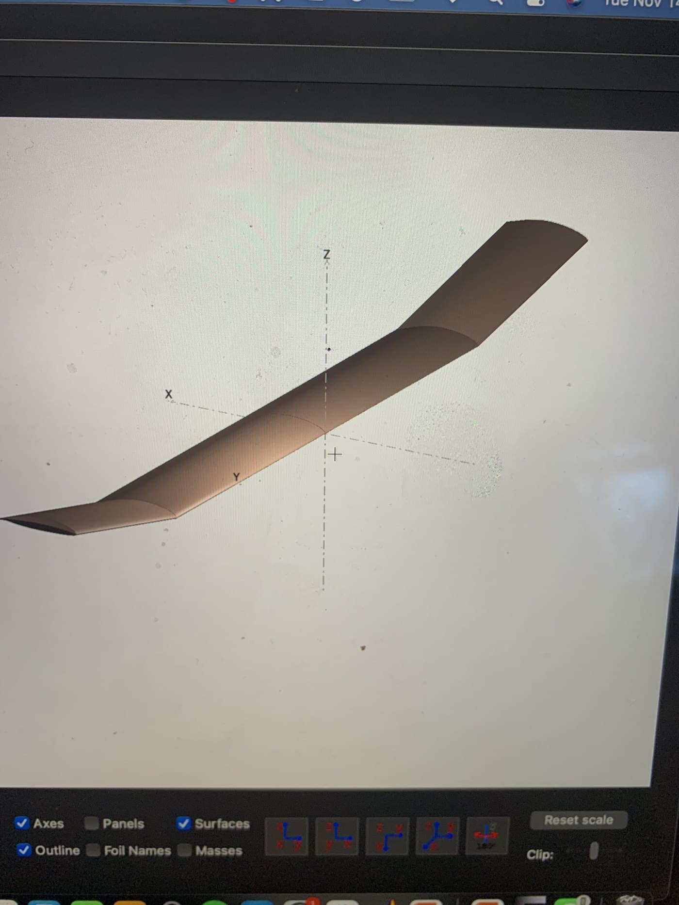
The wing uses two sections of dihedral — 4° on the main section, 16° at the tips — to create a curved-wing effect for lateral stability. Because the spar is angled, we laser-cut it from balsa rather than hardwood, and designed the spar joint with interlocking teeth so the two wing halves and the fuselage lock together rigidly.
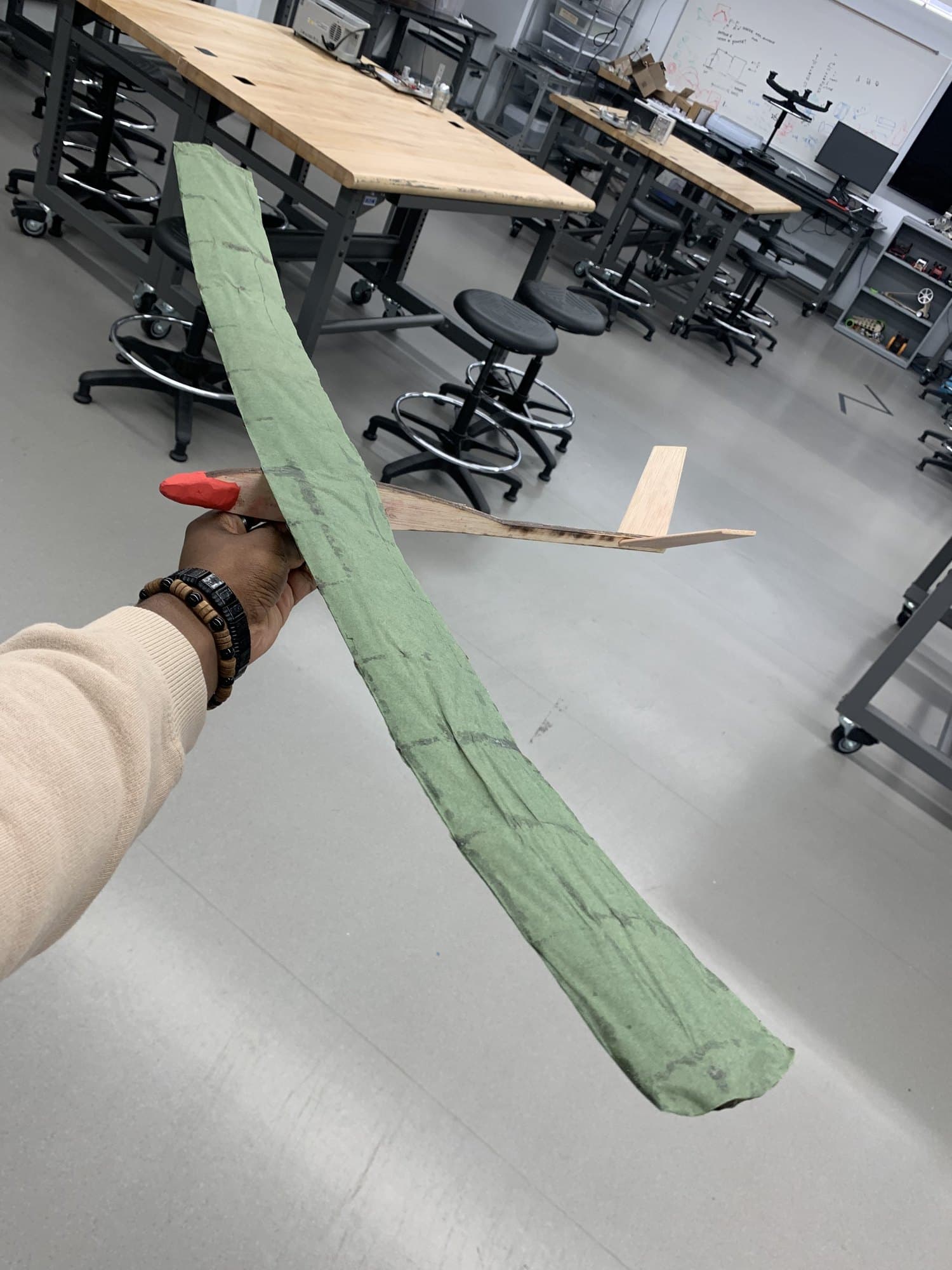
The tail changed between prototypes. Our first design used a V-tail, but angling it precisely proved difficult and it was probably undersized — the glider banked to one side on every flight. We moved to a conventional vertical and horizontal stabilizer for the final build, and added cutouts to the tail and rear fuselage because the initial design pitched up: the centre of mass sat behind the centre of lift.
The fuselage is itself an airfoil section, a Wortmann FX 60-126, so that the roughly 10% of total lift and drag a fuselage typically contributes works in our favour rather than against it.
Analysis and validation
| Parameter | Hand calculation | XFLR5 model |
|---|---|---|
| C_l at α = 0 | 0.371 | 0.41 |
| C_d at α = 0 | 0.0638 | 0.11 |
| C_m at α = 0 | 0 | −0.0005 |
| Flight speed | 5 m/s | 5 m/s |
The simulated lift coefficient sits slightly above the required one, which says the glider can produce the lift it needs and may even fly a little slower than 5 m/s while doing so. The simulated drag coefficient is higher than the hand calculation because the XFLR5 model includes the tail and fuselage rather than the wing section alone — so the disagreement is expected and in the right direction.
Moment coefficients came out near zero across the range, and the root-locus analysis placed every pole of the system in the left half plane. Physically, that means an impulsive disturbance self-corrects back to zero in both pitch and roll — which the impulse response curves confirm directly.
Competition and honest assessment
| Trial | Distance | Time | Average speed |
|---|---|---|---|
| 1 | 9 m | 2.38 s | 3.78 m/s |
| 2 | 13 m | 2.58 s | 5.04 m/s |
| 3 | 16.9 m | 2.90 s | 5.69 m/s |
The glider flew straight and was stable, but after a brief level-flight period it would lose lift and drop before the finish line. Measured glide ratio came out at 4.73 against a theoretical 5.81, and measured sink rate at 1.066 m/s against a theoretical 0.859 m/s — both consistent with real drag exceeding the theoretical estimate. The team placed in the top 5 of more than 30 entries.

Scaling to the fictional atmosphere exposed a second limit. Matching Reynolds number across a 150× density drop and a 1.5× viscosity drop forces a velocity ratio of 14.2 and a length ratio of 7.03, giving a 6 m wingspan flying at 71.1 m/s — Mach 0.59 in that atmosphere, far outside anything a glider does on Earth, and at 2.51 kg too light to carry meaningful instrumentation. The scaled design is a valid similitude result and an invalid aircraft, which is itself the useful finding.