Reinforcement Learning for Wing Kinematics in Hovering Flight
Nonlinear equations of motion, quasi-steady aerodynamics, and a PPO agent
- Role
- Sole author
- Status
- Completed
Headline results
M.Eng. Final Report
The full 66-page report: frame definitions, the symbolic derivation of the equations of motion, the blade-element aerodynamic model, the hover parameter study, and every reinforcement-learning run.
Why flapping flight resists analysis
Flapping-wing flight is governed by highly nonlinear, unsteady aerodynamic interactions that make both analytical modeling and control design difficult. Unlike a fixed wing, the aerodynamic environment a flapping wing sees changes continuously within a single stroke, and the body responds to those forces on the same timescale. There is no clean separation between the aerodynamics and the rigid-body dynamics.
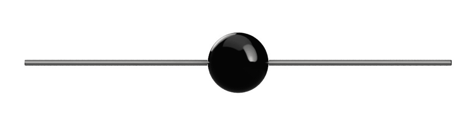
This project builds a reduced-order dynamic model of a flapping system with an ellipsoidal body and rigid wings capable of symmetric flapping and pitching, then asks whether a reinforcement learning agent can discover wing kinematics that hold the body in place.
Deriving the equations of motion
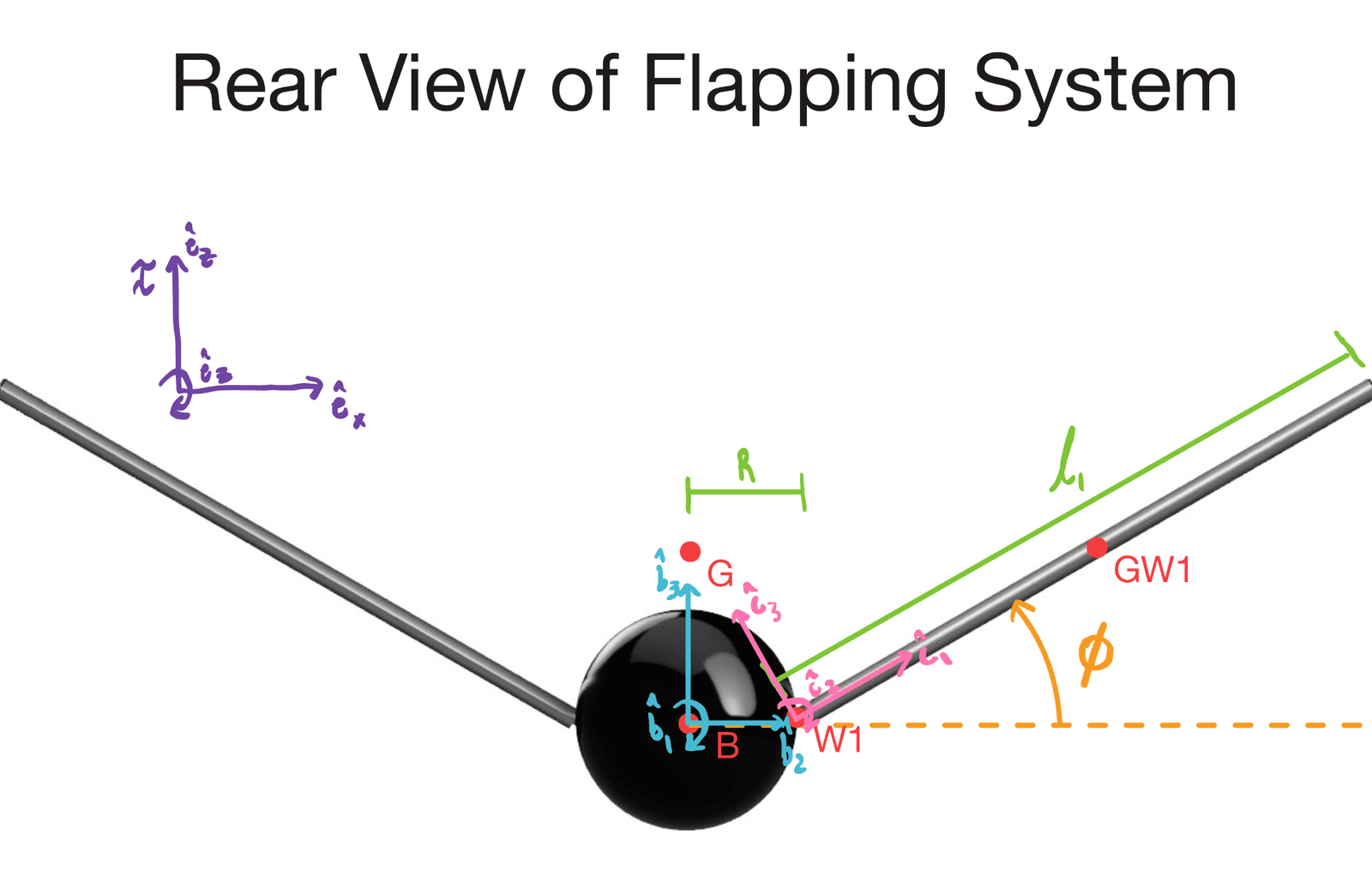
I set up three reference frames — inertial, body, and wing — connected by direction cosine matrices, then applied Newton's second law to the coupled body-plus-wings system. Each wing carries two degrees of freedom, flapping angle φ and pitch angle ψ, pinned at the root. Because the wings carry mass and accelerate relative to the body, the body-frame acceleration terms have to be resolved back into inertial coordinates before the force balance closes.
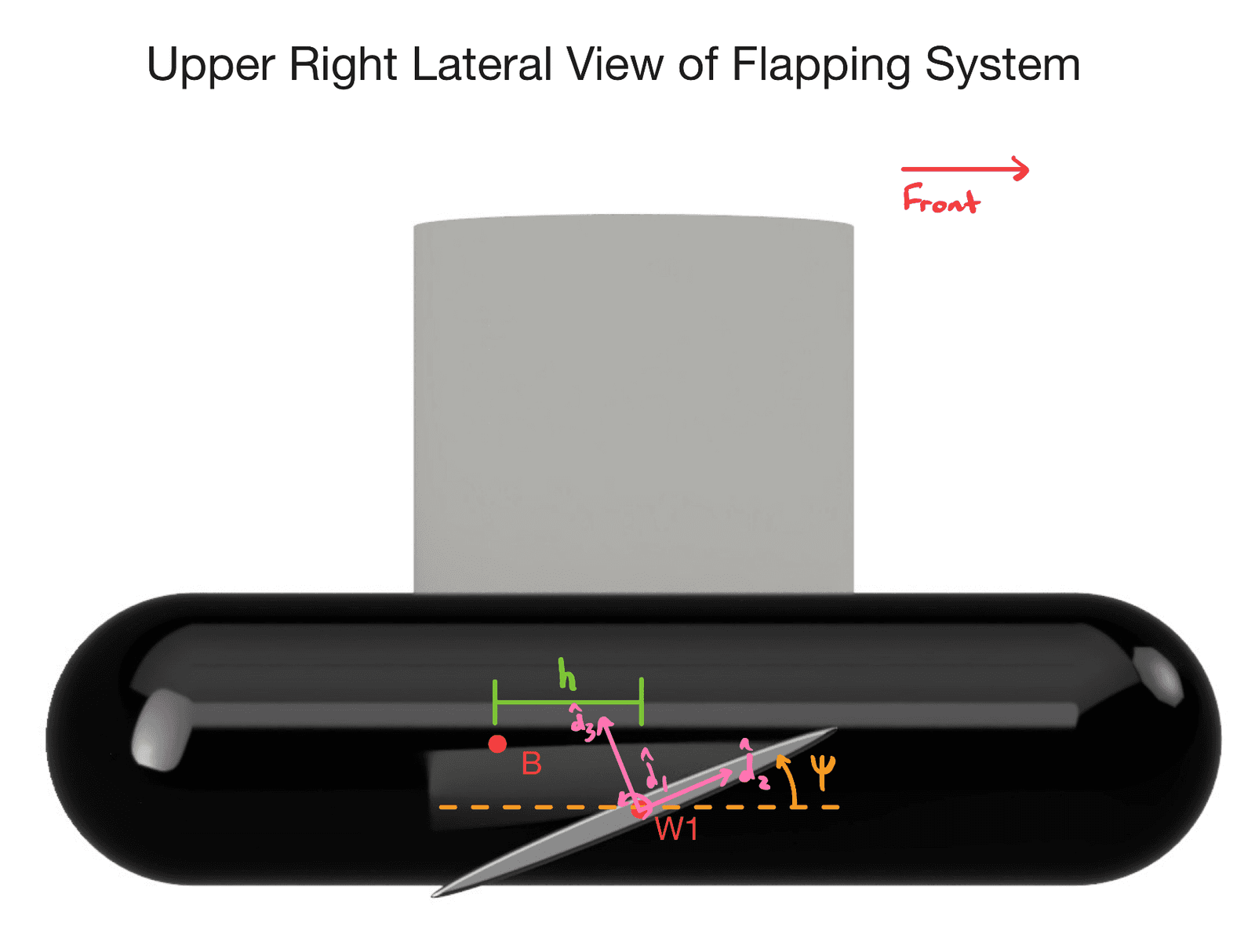
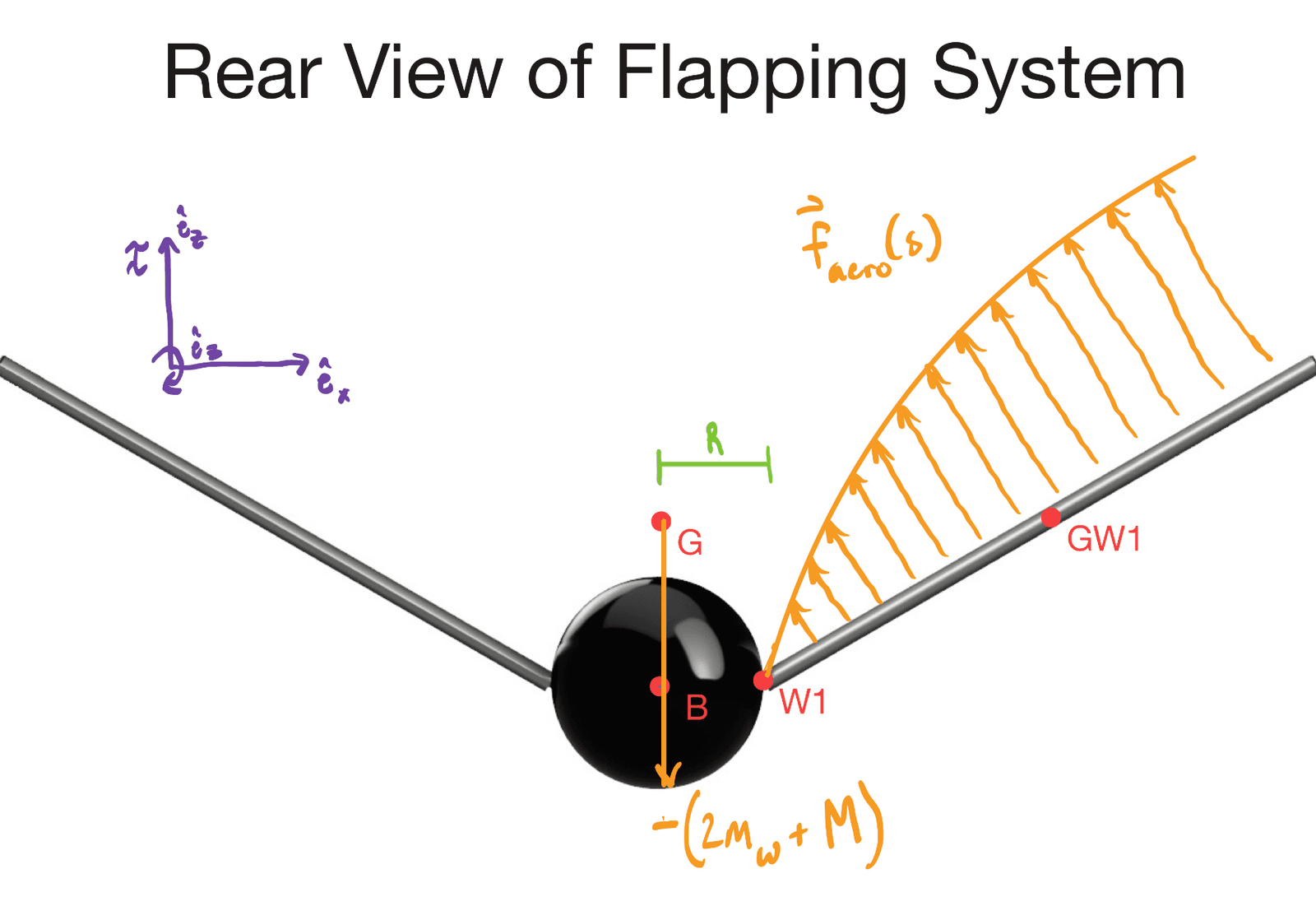
Aerodynamic forces come from a thin-body quasi-steady model in the tradition of Andersen, Pesavento and Wang, applied strip-by-strip along the span and integrated numerically. The symbolic derivation was done in SymPy so the resulting expressions could be differentiated and verified rather than hand-transcribed, and the resulting system is integrated with SciPy's RK45.
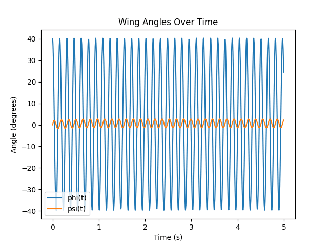
Splitting ψ between upstroke and downstroke — rather than holding pitch constant — is what gives the model control authority over translational motion. The sine form for ψ against the cosine form for φ places maximum pitch at the stroke reversals, where it does the most work.
Finding hover from first principles
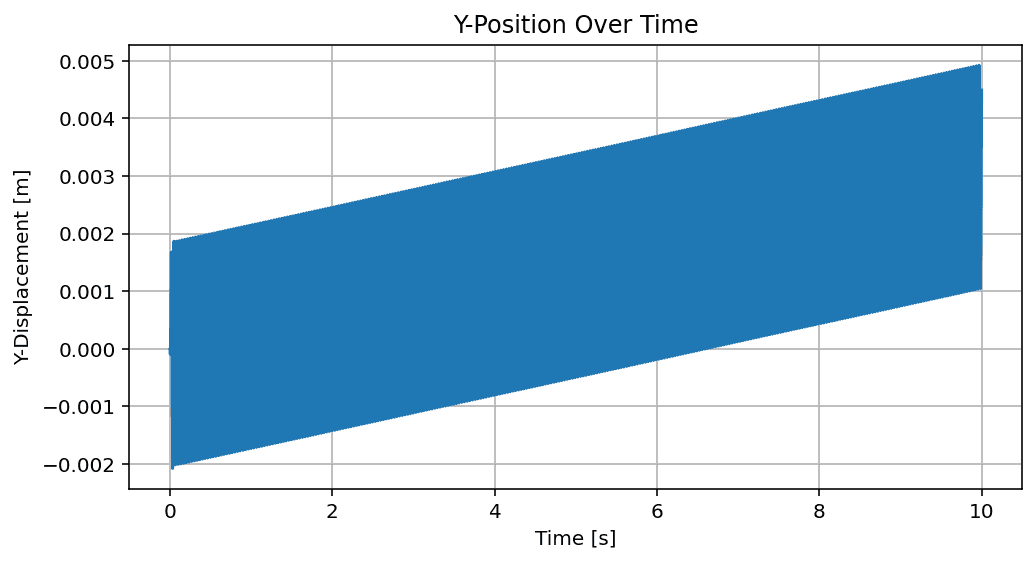
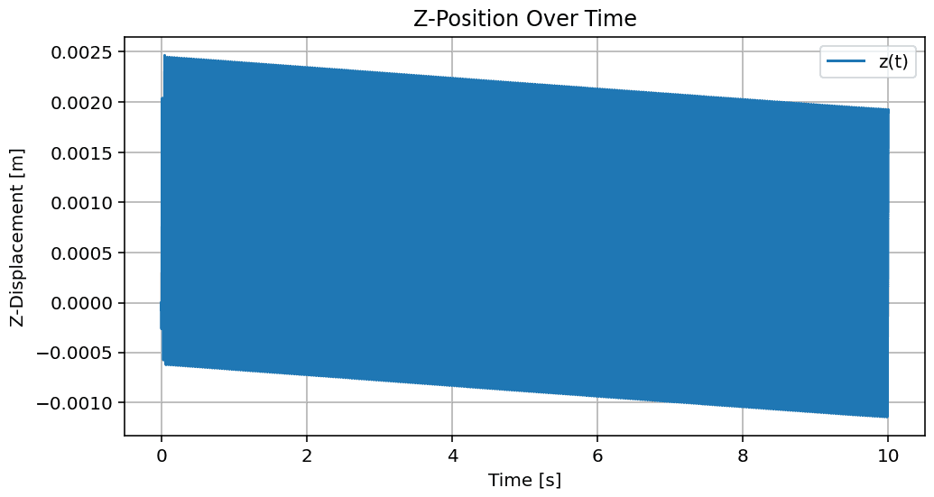
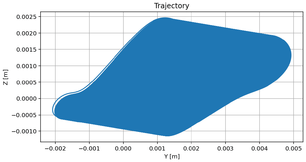
Before handing anything to a learning agent, I validated the equations of motion by sweeping the kinematic parameters directly, using dimensionless coefficients scaled to a housefly. Hovering flight showed up at a specific combination:
The learning environment
I wrapped the simulation in a reinforcement learning environment where the agent adjusts the kinematic parameters — amplitudes, phase offsets, and wingbeat frequency — rather than commanding torques directly. Actions are smoothed between steps so the wing motion stays kinematically continuous instead of jumping discontinuously between wingbeats.
The reward is segment-based: within each evaluation window, a least-squares trend is fit to the body's y and z trajectories, and the agent is penalized on both the intercept difference and the slope difference from the target. Penalizing slope rather than only position is what makes the reward robust to the oscillation inherent in flapping flight — a body that bobs around a fixed point should not be punished the way a body that steadily drifts is.
- Algorithm: Proximal Policy Optimization (PPO), continuous action space
- Physics: full nonlinear EOM integrated in-loop at every environment step
- Aerodynamics: quasi-steady blade element with Gauss–Legendre spanwise integration
- Reward: least-squares trend extraction over trajectory segments, penalizing intercept and slope
Results
The first training attempts did not learn. Both the episode reward mean and the action-distribution standard deviation stayed nearly flat across iterations, which told me the policy was neither exploring nor improving. The problem was conditioning, not capability: the action space was too large and the reward too simply defined for the optimizer to find structure.
Tightening the action bounds and rescaling the reward produced the first genuine learning signal — episode reward rose over 25% and the policy visibly reduced lateral drift. With learning confirmed, I reverted to the originally intended reward formulation and launched a much longer run.
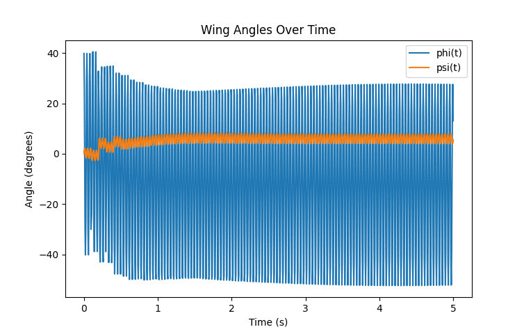
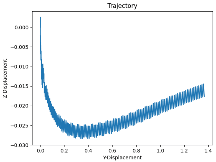
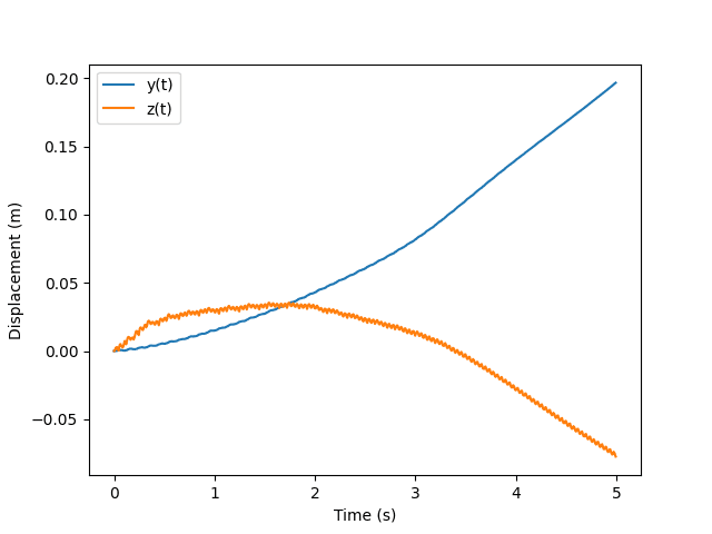
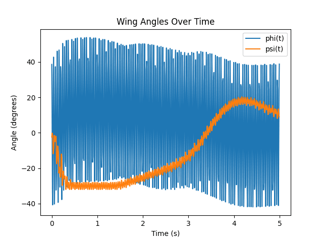
Across roughly 196 iterations of that extended run — about 17 hours of training — the episode reward mean increased by more than 75% while the action distribution standard deviation steadily narrowed. Both signals point the same way: the policy was consistently selecting wingbeat parameters that reduced body drift, and it was becoming more confident about them.
What it did and did not achieve
The PPO agent did not achieve sustained stable hover. It approached it — improving trajectory performance substantially and learning structured, physically plausible flapping motions — but the policy did not converge on the kind of stationary flight the hand-identified kinematics demonstrate.
The most likely cause sits in the reward shaping. Examining the learned kinematics, the reward appears to indirectly over-penalize large amplitudes and high frequencies, which are exactly the regions where hover lives. A policy that is punished for approaching the answer will stop short of it.
This was my first application of reinforcement learning to a physics-driven control problem. Coming from deterministic modeling, rigid-body dynamics, and numerical simulation, integrating policy-based learning and stochastic optimization required stepping well outside my usual analytical framework — which was much of the point.